Author: Ido Greenberg
This post summarizes the work Detecting Rewards Deterioration in Episodic Reinforcement Learning, accepted to ICML 2021. The code is available here.
Introduction
A major challenge in real-world RL is the need to trust the agent, and in particular to know whenever its performance begins to deteriorate. Unlike the framework of many works on robust RL, in real-world problems we often cannot rely on further exploration for adjustment, nor on a known model of the environment. Rather, we must detect the performance degradation as soon as possible, with as little assumptions on the environment as possible. Once detected, corresponding safety mechanisms can be activated (e.g. changing to manual control).
We address this problem in an episodic setup where the rewards within every episode are NOT assumed to be independent, identically-distributed, or based on a Markov process. We suggest a method that exploits a reference dataset of recorded episodes assumed to be “valid”, and detects degradation of rewards compared to this reference dataset.
We show that our test is optimal under certain assumptions; is better than the current common practice even under weaker assumptions; and is empirically better than several alternative mean-change tests on standard control environments – in certain cases by orders of magnitude.
In addition, we suggest a Bootstrap mechanism for False-Alarm Rate control (BFAR), that is applicable to episodic (i.e. non-i.i.d) data.
Our detection method is entirely external to the agent, and in particular does not require model-based learning. Furthermore, it can be applied to detect changes or drifts in any episodic signal.
Why do we need this work?
In Reinforcement Learning (RL) an agent learns a policy to make decisions in various states, leading to collected rewards. The goal of the agent is to maximize the rewards. Many frameworks in RL focus on learning as fast as possible, while losing as little rewards as possible during the process (minimizing the “regret”). This is different from the common framework in many real-world risk-intolerant problems, where the agent must not be modified while running in production. Possible examples are autonomous driving and medical devices (e.g. automatic insulin injection). In such cases, the pipeline may look something like: train -> freeze -> test -> go to production.
What happens if the world changes while the agent runs in production (e.g. unfamiliar weather), or the agent’s own system changes (e.g. worn breaks), or the agent reaches a new, previously unknown domain of states (e.g. new geographic areas)? Certain works considered this question in the context of RL training, usually under restrictive assumptions (e.g. for MDP with known model and specifically-defined modifications of the environment). In such works, the goal is to adjust the training in an online manner. We focus on a different goal – detecting performance degradation following such changes in post-training phase. We aim to address this problem under assumptions as minimal as possible, as required for most real-world problems. In particular, in order not to rely on a state-dependent model, we chose to focus on the distribution of the rewards themselves, as described below.
Once degradation is detected, corresponding safety mechanisms can be activated. For example, the control may pass to a human driver; the patient may be referred to a doctor; a dump may be sent to the developers; etc. The key is to notice the degradation as fast and as reliably as possible. The consequences of late or missing detection may be indicated by the recent accident of a Tesla vehicle with an autopilot module.
Framework
As customary in RL, we assume episodic setup where the agent acts in episodes that differ in their random seeds (that is, in the initial states and possibly in random transitions). Each episode is of length T, and the rewards within the episodes are drawn from some unknown joint distribution over R^T. In particular, the rewards are NOT assumed to be independent of each other, identically-distributed over the episode, or generated by a Markov process.
Our two main assumptions are that:
- The episodes themselves are i.i.d.
- There exists an available reference dataset of recorded episodes with “valid” rewards (e.g. the test period before the marketing of the product).
Note that the agent is fixed during both the reference episodes and the monitoring that comes after that (“post-training” phase).
Solution
The basic suggested approach is very straight-forward: once in a while (e.g. several times per episode) look at the last few episodes, and if the rewards are significantly lower than these of the reference data – declare a degradation.
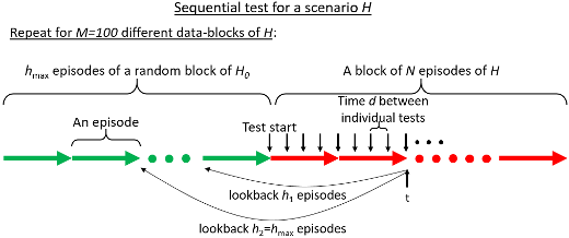
The diagram below describes a framework that tests this approach over N episodes of a modified environment H (compared to the original environment H0; the notations come from the terminology of hypothesis testing). The environment modification is supposed to cause degradation in the agent performance, since the agent is not trained on the modified environment. The better the monitoring algorithm, the sooner we expect to detect this degradation.
Our work addresses two major issues regarding this approach:
- How to “summarize” the rewards (i.e. what is the test-statistic)?
- What is “significantly lower” (i.e. how to choose the test-threshold)?
Test statistic
The natural statistic for comparison of rewards between two groups of episodes is the mean reward. However, by presenting the problem as multivariate mean-shift detection with possibly partial observations, we show that this naive approach is highly sub-optimal. We also consider the mean-shift in a way that corresponds to deterioration of a temporal signal (such as agent rewards), and derive an optimal statistical test for this scenario, which turns out to be simply a weighted mean (unlike standard multivariate mean-shift tests, e.g. Hotelling test).
More specifically, we use the reference dataset to estimate the covariance matrix of the rewards (that is, the variance of the rewards in every times-step, and the correlation between different time-steps), and we define the weights to be the sums of the rows of the inverse covariance matrix.
We prove that:
- If [the deterioration in the rewards is uniform over the time-steps] and [the rewards are multivariate-normal], then this test is optimal (in terms of statistical power).
- We also suggest a near-optimal test for a certain case of non-uniform degradation (see “partial degradation” in the paper).
- Without the normality assumption, the test is still better than the simple mean.
- We also show how much better: roughly speaking, the advantage increases along with the heterogeneity of the eigenvalues of the covariance matrix.
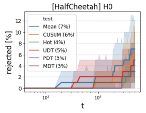
We tested our method on several modified variants of Pendulum, HalfCheetah and Humanoid, as described in the paper. We tested 3 variants of our method: optimal test for uniform degradation (UDT); optimal test for partial degradation (PDT); and a “mix” of PDT and standard tests (MDT). These were tested against 3 conventional tests for mean change: simple mean (Mean), CUSUM test, and Hotelling test (Hot). A sample of the results is shown below.
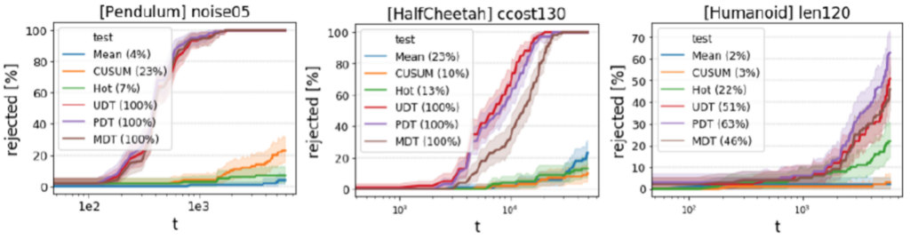
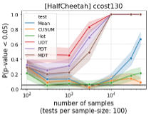
The results above refer to the cumulative number of detections over a sequential test. Consider instead a setup of individual (not sequential) test, where we are given a sample of rewards and need to decide whether they came from a “bad” (i.e. modified) environment. In this setup we encounter a very interesting phenomenon, as demonstrated in the figure below: the tests that do not exploit the covariance matrix “correctly”, sometimes suffer from decrease in detection rates during the first episode, which is not fully recovered even after numerous episodes. In other words, these tests do better with the several first time-steps than they do with the data of several whole episodes! Our tests, on the other hand, usually show increasing performance with the amount of data, as expected from a data-driven statistical test.
Threshold tuning
In the test described above we (repeatedly) calculate a function of the rewards (e.g. weighted mean), and test whether it is too small. In hypothesis testing, “too small” usually means: “so small, that if the environment were valid and not modified, then observing such small rewards just by bad luck would have probability smaller than alpha“. In other words, on a valid environment, the test returns a false-alarm with probability alpha.
If the distribution of the test statistic (for a valid environment) is known, then we can simply take its alpha percentile as the test-threshold, and it is guaranteed to satisfy the condition described above. In cases where the distribution is not known, it is common to use sampling based on bootstrap or Monte-Carlo method in order to approximate the distribution of the statistic. However, the rewards in our case are not i.i.d, while numerical methods usually rely on the data-samples being i.i.d in order to simulate new datasets by re-sampling.
In the context of sequential tests, where tests are applied repetitively, it is common to refer to the “false-alarm rate”, that is, the amount of time between false-alarms. In our work we tune the test-threshold according to the criterion: “during h episodes of test on a valid environment, raise a false-alarm with probability lower than alpha“. Many methods exist for tuning of tests-thresholds in sequential tests. However, even the methods that permit overlapping data between consecutive tests, usually do not permit correlated data as in our case.
We suggest a Bootstrap mechanism for False-Alarm Rate control (BFAR) that overcomes both difficulties described above. The mechanism relies on the assumption that even though the time-steps are not i.i.d, the episodes are. It handles tests of various lengths, including in the middle of episodes, and also supports tuning of thresholds for multiple tests that run in parallel (as used both by the MDT test mentioned above, and by multi-horizon tests as shown in the diagram above).
The figure below demonstrates the success of the threshold tuning in HalfCheetah environment: when running on the valid environment (i.e. without modifications), each of the various test methods has false-alarms in approximately 5% of the 50-episodes-long sequential tests.