Distributional Policy Optimization: An Alternative Approach for Continuous Control

Chen Tessler*, Guy Tennenholtz* and Shie Mannor
Published at NeurIPS 2019
Paper, Code

What?

We propose a new optimization framework, named Distributional Policy Optimization (DPO), which optimizes a distributional loss (as opposed to the standard policy gradient).

As opposed to Policy Gradient methods, DPO is not limited to parametric distribution functions (such as Gaussian and Delta distributions) and can thus cope with non-convex returns

Author: Chen Tessler @tesslerc

Why?

The policy gradient
\(\theta_{k+1} = \theta_k + \alpha_k \mathbb{E}_{s\sim d(\pi_{\theta_k})} \mathbb{E}_{a\sim \pi_{\theta_k}(\cdot|s)} \nabla_\theta \log \pi_\theta (a|s) \mid_{\theta = \theta_k} Q^{\pi_{\theta_k}} (s, a)\) calculates the gradient of \(\theta\) by multiplying the gradient of the log probability of the action taken, by its value. Intuitively, the policy gradient will shift the distribution such that it will induce a higher value (give better actions a higher probability). As the gradient requires the probability of an action being taken, policy gradient methods are limited to parametric distribution functions, in which we can directly calculate the PDF (probability density function), i.e., obtain the probability of an action.

However, the policy gradient approach has a major limitation. Consider the following action-value function:

A non-convex optimization landscape — A general non-convex objective

As, in our Gaussian example, the gradient directly controls \(\mu\) and \(\sigma\), a small movement of \(\mu\) to the left will result in a decrease in the attained value. As such, in this example, this local movement limitation causes the policy to shift to the right – resulting in convergence to a sub-optimal local-extremum. As shown in the figure below.

PPO converges to a sub-optimal solution — PPO Converges to a sub-optimal solution

Due to the limitation to Gaussian policies, the approach is incapable of converging to the global optimum, while policy gradient approaches over the set of entire policies are ensured (in the tabular case) to converge to a global optima

The figure above illustrates this theoretical issue.

The optimal approach, depicted on the left (and show in the figure below), would be to calculate the gradient with respect to the policy itself (i.e., in the probability space \(\Pi\)). However, in practice, due to the limitation of residing within the set of probability distributions \(\Theta\) (e.g., the set of Gaussian distributions), it may converge to a sub-optimal local-extrema.

Sought after behavior - moving probability mass towards the argmax — Sought after behavior – moving probability mass towards the argmax

How?

Recall that the policy gradient is limited to parametric distributions (e.g., Gaussian and Delta functions), as it requires the ability to directly calculate the probability of an action being performed. In DPO we propose an alternative, fundamentally different, yet simple approach.

Policy learning procedures follow a simple learning paradigm, in which at each step a new policy is found such that it improves over the previous one. The value of such an approach has a single fixed-point and is thus ensured to converge to a globally optimal solution.

DPO follows a similar procedure. Given a previous policy \(\pi\), DPO defines the next policy as some probability distribution over the actions which have a positive advantage, where the advantage is defined as:

\(A^\pi (s,a) = Q^\pi (s, a) – v^\pi (s)\)

This iterative procedure ensures that at each step the following policy will improve upon the previous one, such that the same asymptotic convergence holds, as in the classic policy learning algorithms.

DPO is presented in Algorithm 1. It is composed of 4 components learning in parallel.

The target policy \(\pi’\) (line 5), which follows the policy \(\pi\) “slowly”.

The action-value function \(Q\)

and the value function \(v\), both of which estimate the utility of the target policy \(\pi’\).

The policy \(\pi\) (line 2), which converges towards a distribution over the positive advantage of the target policy \(\pi’\).

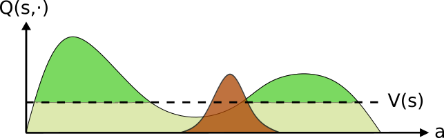
This procedure is illustrated in the following figures. We start with an initial policy (brown) and estimate both it’s \(Q\) (the curved line) and \(v\) (the dashed line) values. We then define the positive advantage (green) as the actions which obtain a higher outcome than the expectation over the policy (the value \(v\)).

(1) Beginning with an initial policy, it's evaluated performance is denoted by V (the vertical dotted line) and the improving actions (those with positive advantage) in green — (1) Beginning with an initial policy, it’s evaluated performance is denoted by V (the vertical dotted line) and the improving actions (those with positive advantage) in green

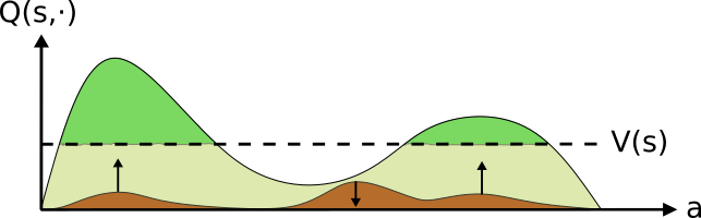
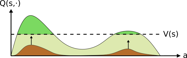
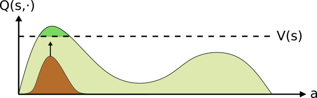
The policy is then updated towards a distribution over the actions with a positive advantage. This can be seen as moving probability mass from “bad” actions towards “better” ones. This iterative scheme continues until convergence is obtained.

Once the advantage is calculated, DPO defines the objective in distribution space. E.g., the loss minimizes the distance between the target distribution (fixed) and the policy (trainable). This is akin to moving probability mass from the "bad" actions towards those which are "good" — Once the advantage is calculated, DPO defines the objective in distribution space. E.g., the loss minimizes the distance between the target distribution (fixed) and the policy (trainable). This is akin to moving probability mass from the “bad” actions towards those which are “good”

DPO performs this iterative approach, continuing to improve

As DPO considers all actions and is not bounded to a fixed distribution class, it's fixed point (in theory) is a global extrema — As DPO considers all actions and is not bounded to a fixed distribution class, it’s fixed point (in theory) is a global extrema

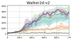
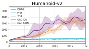
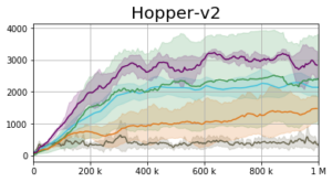
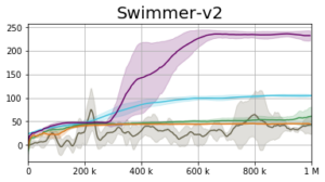
Experiments

Our empirical approach to tackling the DPO optimization problem is named the Generative Actor Critic (GAC). The actor is represented using an Implicit Quantile Network [6, 7] and optimized using the quantile regression loss [8, 9]. Our results are presented below. GAC Linear (AIQN) and GAC Boltzmann (AIQN) represent the results of the autoregressive implementation in which the distribution over the positive advantage is defined using a linear

\(\frac{A^\pi (s,a)}{\int_{I^\pi(s)} A^\pi (s,a’)da’}\)

or a Boltzmann distribution

\(\frac{exp(\frac{1}{\beta}A^\pi (s,a))}{\int_{I^\pi(s)} exp(\frac{1}{\beta}A^\pi (s,a’))da’}\)

The GAC Boltzmann (IQN) shows the scenario in which we do not model the inner-action dependencies (i.e., without using an autoregressive model).

Conclusions

In this work we presented limitations inherent to empirical Policy Gradient (PG) approaches in continuous control. While current PG methods in continuous control are computationally efficient, they are not ensured to converge to a global extrema. As the policy gradient is defined w.r.t. the log probability of the policy, the gradient results in local changes in the action space (e.g., changing the mean and variance of a Gaussian policy). These limitations do not occur in discrete action spaces.

We suggested the Distributional Policy Optimization (DPO) framework and its empirical implementation – the Generative Actor Critic (GAC). We evaluated GAC on a series of continuous control tasks under the MuJoCo control suite. When considering overall performance, we observed that despite the algorithmic maturity of PG methods, GAC attains competitive performance and often outperforms the various baselines. Nevertheless, there is “no free lunch” [10]. While GAC remains as sample efficient as the current PG methods (in terms of the batch size during training and number of environment interactions), it suffers from high computational complexity.

Bibliography

[1] Richard S Sutton, David A McAllester, Satinder P Singh, and Yishay Mansour. Policy gradient methods for reinforcement learning with function approximation. InAdvances in neural information processing systems, pages 1057–1063, 2000.

[2] https://lilianweng.github.io/lil-log/2018/04/08/policy-gradient-algorithms.html

[3] Ian Goodfellow, Jean Pouget-Abadie, Mehdi Mirza, Bing Xu, David Warde-Farley, Sherjil Ozair, Aaron Courville, and Yoshua Bengio. Generative adversarial nets. InAdvances in neural information processing systems, pages 2672–2680, 2014.

[4] Diederik P Kingma and Max Welling. Auto-encoding variational bayes. arXiv preprint arXiv:1312.6114, 2013.

[5] Will Dabney, Mark Rowland, Marc G Bellemare, and Remi Munos. Distributional reinforcement learning with quantile regression. arXiv preprint arXiv:1710.10044, 2017.

[6] Will Dabney, Georg Ostrovski, David Silver, and Remi Munos. Implicit quantile networks for distributional reinforcement learning. arXiv preprint arXiv:1806.06923, 2018a.

[7] Georg Ostrovski, Will Dabney, and Remi Munos. Autoregressive quantile networks for generative modeling. arXiv preprint arXiv:1806.05575, 2018.

[8] Roger Koenker and Kevin Hallock. Quantile regression: An introduction. Journal of Economic Perspectives, 15(4):43–56, 2001.

[9] Roger Koenker and Zhijie Xiao. Quantile autoregression. Journal of the American Statistical Association, 101(475):980–990, 2006.

[10] David H Wolpert, William G Macready, et al. No free lunch theorems for optimization. IEEE transactions on evolutionary computation, 1(1):67–82, 1997.